Getting started with EraBrewer

EraBrewer provides color palettes inspired by Taylor Swift’s albums. This vignette walks through the two main ways to use them in a ggplot2 workflow: as a discrete scale (one color per category) and as a continuous scale (a smooth gradient over a numeric variable). For each palette we then pair the canonical scatter plot with a second geom that matches that scale — a bar chart for the discrete case, and a diverging heatmap for the continuous case.

library(EraBrewer)
library(ggplot2)

Step 1 — Picking palettes

All available palettes live in the exported list EraPalettes:

names(EraPalettes)
#>  [1] "Red1"               "Red2"               "NineteenEightyNine"
#>  [4] "Showgirl1"          "Showgirl2"          "SpeakNow1"         
#>  [7] "SpeakNow2"          "TorturedPoet"       "Fearless"          
#> [10] "Evermore1"          "Evermore2"          "Reputation"        
#> [13] "Lover1"             "Lover2"             "TaylorSwift"       
#> [16] "Midnight1"          "Midnight2"

We pick one palette to use discretely and one to use continuously:

discrete_pal   <- era.brewer("Lover2",    n = 3)
continuous_pal <- era.brewer("Midnight2", n = 100, type = "continuous")

era.brewer() returns a "palette" object — a character vector of hex codes with a print() method that returns a ggplot swatch.

print(era.brewer("Lover2")) + transparent_theme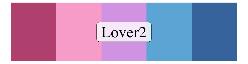

print(era.brewer("Midnight2")) + transparent_theme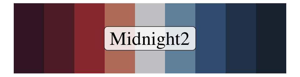

When type = "discrete" (the default whenever n does not exceed the palette length), era.brewer() returns the colors hand-picked by the palette’s curator as the best subset of that size. When type = "continuous", it interpolates the stored colors with grDevices::colorRampPalette() to produce as many shades as you ask for.

Step 2 — A discrete scale (Lover2)

For the discrete case we color by Species in iris and feed the palette to scale_color_manual() / scale_fill_manual() via the values argument.

Scatter plot

ggplot(iris, aes(Sepal.Length, Sepal.Width, color = Species)) +
  geom_point(size = 2.4, alpha = 0.9) +
  scale_color_manual(values = discrete_pal) +
  labs(title = "Iris sepals, colored by species",
       x = "Sepal length (cm)", y = "Sepal width (cm)")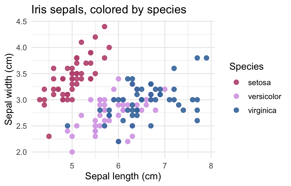

Bar chart

species_means <- aggregate(Sepal.Length ~ Species, iris, mean)

ggplot(species_means, aes(Species, Sepal.Length, fill = Species)) +
  geom_col(width = 0.65) +
  scale_fill_manual(values = discrete_pal) +
  labs(title = "Mean sepal length by species",
       x = NULL, y = "Sepal length (cm)") +
  theme(legend.position = "none")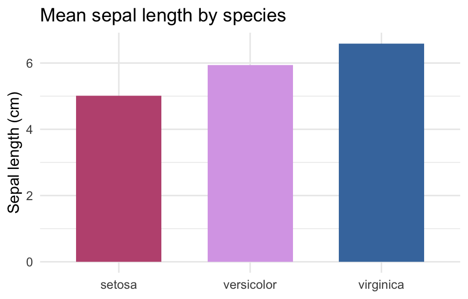

Step 3 — A continuous scale (Midnight2)

Midnight2 runs from a warm red through a neutral gray to a cool blue, which makes it a natural fit for quantities that are signed or otherwise diverging around a meaningful center. We use it on a numeric color aesthetic via scale_color_gradientn() / scale_fill_gradientn(), passing the interpolated palette through colors =.

Scatter plot

ggplot(iris, aes(Sepal.Length, Sepal.Width, color = Petal.Length)) +
  geom_point(size = 2.4, alpha = 0.95) +
  scale_color_gradientn(colors = continuous_pal) +
  labs(title = "Iris sepals, shaded by petal length",
       x = "Sepal length (cm)", y = "Sepal width (cm)",
       color = "Petal length")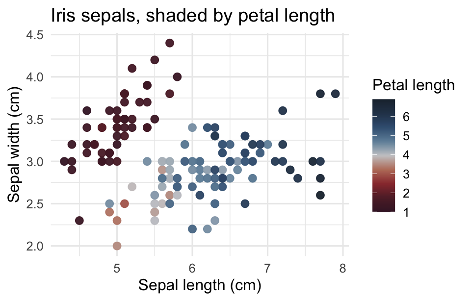

Diverging heatmap

A correlation matrix is the canonical case for a diverging palette: the values live in [-x, x], the sign carries meaning, and zero is the neutral midpoint we want mapped to the palette’s gray center.

cor_mat <- cor(mtcars)
cor_df  <- as.data.frame(as.table(cor_mat))
names(cor_df) <- c("Var1", "Var2", "rho")

ggplot(cor_df, aes(Var1, Var2, fill = rho)) +
  geom_tile(color = "white", linewidth = 0.4) +
  scale_fill_gradientn(colors = continuous_pal,
                       limits = c(-1, 1),
                       breaks = c(-1, -0.5, 0, 0.5, 1)) +
  coord_fixed() +
  labs(title = "mtcars correlation matrix",
       x = NULL, y = NULL, fill = expression(rho)) +
  theme(axis.text.x = element_text(angle = 45, hjust = 1),
        panel.grid  = element_blank())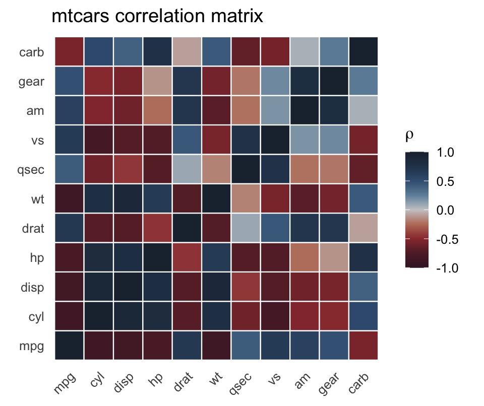

Recap

	Scatter (color = …)	Companion geom
Discrete	scale_color_manual(values = era.brewer("Lover2", n = 3))	Bar chart with scale_fill_manual()
Continuous	scale_color_gradientn(colors = era.brewer("Midnight2", n = 100, type = "continuous"))	Diverging heatmap with scale_fill_gradientn(limits = c(-1, 1))

Notes:

• direction = -1 reverses the palette.
• override_order = TRUE returns the colors in storage order instead of our preferred order-of-use (only relevant for discrete palettes).
• If you request more colors than a palette holds, era.brewer() switches to "continuous" automatically.